
SQL for Tableau: Window Functions

It’s been a while since I’ve shared a blog in my SQL
for Tableau Users series, so I’m excited to be back with a blog on one of my
absolute favorite features of SQL, window functions!! OK, they may not sound
that exciting but they are really powerful and, once you get the syntax down,
relatively easy to write.
Let’s start out by defining window functions. I personally like
the definition provided by the PostgreSQL
documentation:
A window function performs a calculation across a set of table
rows that are somehow related to the current row. This is comparable to the
type of calculation that can be done with an aggregate function. But unlike
regular aggregate functions, use of a window function does not cause rows to
become grouped into a single output row—the rows retain their separate
identities. Behind the scenes, the window function is able to access more than
just the current row of the query result.
OK, that’s a bit confusing, but it’ll become much clearer as we
look at some examples. So let’s start by looking at a simple example using
Superstore on my publicly-available SQL Server (see SQL
for Tableau Part 1: The Basics for details on
connecting to this server).
We’ll begin with a simple aggregation of sales by region.
SELECT [Region], SUM([Sales])
FROM [Orders]
GROUP BY [Region]

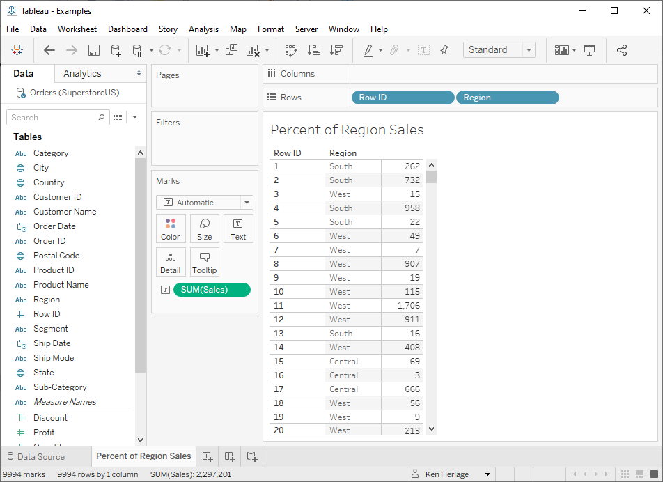
We get one record for each region with each region’s total
sales. But what if we want to see every row along with the sum of sales for the
region?
SELECT [Row ID], [Region], [Sales],
SUM([Sales]) OVER (PARTITION BY [Region]) AS [Region Sales]
FROM [Orders]

The second line of the SQL leverages a window function to
provide us with data outside of the row we’re looking at.
Let’s take a look at the the syntax:
SUM([Sales]) OVER (PARTITION BY [Region])
This statement starts with a function—in this case, an
aggregation—then is followed by OVER. OVER essentially tells the database that
we’re about to define the window. Then, within parentheses, we define the
window using the PARTITION BY clause. This tells the database that we want to
partition (i.e. group) our records together by the Region. So, in plain
English, this would say “Sum the sales for the entire region that is specified
on this row.”
Note: If you do not
wish to partition your data at all (i.e. get the total sales for the entire
data set), then you would simply not include the PARTITION BY clause:
SUM([Sales]) OVER () AS [Region Sales]
What’s nice about this is that it allows us to then perform some
additional aggregations. For example, we could find each row’s percentage of
the region’s sales.
SELECT [Row ID], [Region], [Sales]/SUM([Sales]) OVER (PARTITION BY [Region]) AS [% of Sales]
FROM [Orders]

To take this one step further, we can aggregate the main query
as well. For example, let’s say we want to see the percentage of sales by
customer, rather than each individual row. To do that, we’ll need to aggregate
the sales by customer then divide by the total regional sales:
SELECT [Region], [Customer Name],
SUM([Sales]) AS [Customer Sales],
SUM(SUM([Sales])) OVER (PARTITION BY [Region]) AS [Region Sales]
FROM [Orders]
GROUP BY [Region], [Customer Name]

Notice that we need to further aggregate the window calculation.
Without it, we’ll get an error. I won’t show you here, but you can see that we
could now easily calculate the percent of regional sales for each customer.
Similarity to Tableau
If the above feels familiar to you, that’s because you’ve
probably done something very similar in Tableau. Let’s take the above use case
(each record’s percent of regional sales) and use Tableau to solve it. To do
this, we’d use either LODs or window calculations. Let’s begin with window
calcs. We’d start by creating our basic view:
Then we could write a calculation like this:
Region Sales
// Sales for the overall region.
WINDOW_SUM(SUM([Sales]))
Then we add this to the view, make sure it’s set to compute
properly, and we’ll get:
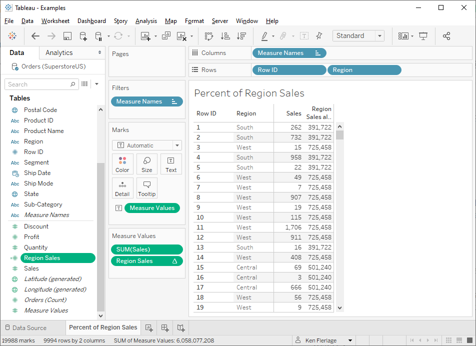
Then, of course, we could perform the math, SUM([Sales])/[Region
Sales] to get the percentage.
If we examine this closely, we can see how similar the SQL window
functions are to this window SUM. Let’s look at them together:
SUM(SUM([Sales])) OVER (PARTITION BY [Region])
WINDOW_SUM(SUM([Sales]))
We don’t have to tell SQL that it’s a window calculation because
of the OVER clause, whereas Tableau needs to know that we’re using a window
sum. Additionally, in SQL, we specify how to partition our data within the
script, while in Tableau, we specify this partitioning when we tell it how to
compute the table calculation.
........................
A second option for doing this in Tableau would be an LOD
calculation. Instead of the window sum, we’d do the following:
Region Sales
// Sales for the overall region.
{FIXED [Region]: SUM([Sales])}
This will produce the same result as our table calc. While this
is syntactically less similar to the SQL than the window sum, we can definitely
see some similarities. Fixing on Region in the LOD is similar to partitioning
on Region in the SQL. Then, of course, we’re summing the sales within that
partition.
Interestingly, the definition of window calculations shared
earlier included the following: “Behind the scenes, the window function is able
to access more than just the current row of the query result.” That sounds a
lot like an LOD calculation and, as we’ve seen, they have a lot of
similarities.
It’s important to point
out that neither Tableau window calcs nor LODs are exactly synonymous with SQL
window calcs. These Tableau calculations can change based on the dimensions on
your view, the way you set them up to be computed, filters, and a number of
other things. However, there are a lot of similarities, so considering your
likely familiarity with these concepts already, I think they are valuable to
help illustrate how SQL window calcs work.
Order By
We’ve seen how we can use PARTITION BY to partition our window
functions, but there’s also another part of the syntax that can be very
valuable, ORDER BY. To demonstrate this, let’s take a look at a scenario where
we’d like to number each record. To do this, we can use the window function,
ROW_NUMBER:
SELECT [Row ID], [Region], [Customer Name],
ROW_NUMBER() OVER (ORDER BY [Row ID]) AS [Row]
FROM [Orders]

In this case, we’re telling the database to give us a sequential
row number ordered by Row ID. Since Row ID is a sequential number already, it’s
not surprising that we get the same value. However, we can do a variety of
other things, including changing the sort order. Just like normal ORDER BY
statements, the data is sorted ascending by
default, but if we add DESC after the sort, it’ll sort descending.
SELECT [Row ID], [Region], [Customer Name],
ROW_NUMBER() OVER (ORDER BY [Row ID] DESC) AS [Row]
FROM [Orders]

We can also sort on multiple fields. For example, let’s say we
wish to number our rows first by Region, then by Sales from highest to lowest.
SELECT [Row ID], [Region], [Customer Name], [Sales],
ROW_NUMBER() OVER (ORDER BY [Region] ASC, [Sales] DESC) AS [Row]
FROM [Orders]

We’ve now essentially ranked our data for each region. Or did
we? If we scroll down to the point where it changes from the Central region to
the East, we can see what might be a problem (depending on our goal).

In this case, it just continues to number the records once it
gets to a new region. But what if we want it to start over at each region (just
like we might do with the “Restarting every” option of a Tableau table
calculation)? This is where we can reintroduce PARTITION BY.
SELECT [Row ID], [Region], [Customer Name],
ROW_NUMBER() OVER (PARTITION BY [Region] ORDER BY [Region] ASC, [Sales] DESC) AS [Row]
FROM [Orders]

Because we’ve told the database to partition by the Region, it
will restart the numbering when a new Region is encountered. While rudimentary,
this works as a basic ranking mechanism, showing us the rank of each record
within its given region.
While I’m here, I think
it’s important to point out the similarity in this syntax to Tableau Prep’s new
analytic functions. One of the fantastic
functions they’ve made available is none other than ROW_NUMBER. In Prep, you’d
perform this same basic row numbering technique using the following syntax:
{PARTITION [Region]: {ORDERBY [Region] ASC, [Sales] DESC : ROW_NUMBER()}}
This syntax is very
similar to what we use in SQL, down to the key words used (PARTITION,
ORDERBY)—even more so than the window calcs and LODs we discussed earlier.
Additional Functions
There are a handful of additional window functions that we have
not yet discussed, two are which are my absolute favorite (I’ll save them for
last). So, here are a few of them, with examples:
RANK/DENSE_RANK
Not surprisingly, this will rank your data. So, instead of the
row numbering method used above, we could write this:
SELECT [Row ID], [Region], [Customer Name],
RANK() OVER (PARTITION BY [Region] ORDER BY [Region] ASC, [Sales] DESC) AS [Row]
FROM [Orders]

Unlike the row number function, rank handles ties by giving both
rows the same rank (just like the RANK function in Tableau). There is also a
variant of this, DENSE_RANK, which works just like Tableau’s RANK_DENSE
function.
FIRST_VALUE/LAST_VALUE
These will return the first or last value within a partition.
For example, let’s say that you want to compare a customer’s sale to that
customer’s first ever sale. Without
window functions, this is pretty difficult and requires various sub-queries,
but FIRST_VALUE makes it much easier.
SELECT [Row ID], [Customer Name], [Order Date], [Sales],
FIRST_VALUE([Sales]) OVER (PARTITION BY [Customer Name] ORDER BY [Order Date]) AS [First Sale Amount]
FROM [Orders]

Likewise, we can use LAST_VALUE to obtain the last value in the
partition.
LEAD/LAG
OK, now for my favorite window functions, LEAD and LAG. LEAD
allows you to get a value from a later row in the data set, while LAG allows
you to get a value from a previous row. For example, the following SQL will get
a customer’s prior and next sales amount:
SELECT [Customer Name], [Row ID], [Order Date], [Sales] ,
LAG([Sales]) OVER (PARTITION BY [Customer
Name] ORDER BY [Customer Name], [Order Date]) AS [Prior Sales],
LEAD([Sales]) OVER (PARTITION BY [Customer Name] ORDER BY [Customer Name], [Order Date]) AS [Next Sales]
FROM [Orders]

Though not shown in the above example, the LEAD and LAG
functions have two additional parameters—offset and default value. Offset
allows you to specify the number of rows back or forward you move, while the
default value allows you to specify a value to return when we are outside of a
partition. For instance, the NULL values in the above example—using Customer
Name as a partition—result from the fact that the customer does not have a
previous or next record.
We could, for example, write the following which will move
backward and forward by 2 rows and return 0 as a default.
SELECT [Customer Name], [Row ID], [Order Date], [Sales] ,
LAG([Sales], 2, 0) OVER (PARTITION BY [Customer
Name] ORDER BY [Customer Name], [Order Date]) AS [Sales 2 Back],
LEAD([Sales], 2, 0) OVER (PARTITION BY [Customer Name] ORDER BY [Customer Name], [Order Date]) AS [Sales 2 Fwd]
FROM [Orders]

The reason I love these functions so much is that they have a
ton of different use cases. Often, we find ourselves leveraging the LOOKUP
function in Tableau to perform this operation. While that can often give us the
correct results, having these values on a single record provides us so much
more flexibility since it allows us to perform row-level calculations, avoiding
the more complex table calculations.
For a great example of the power of LEAD and LAG, check out the
blog I co-authored with fellow Tableau Zen Master, Klaus Schulte: Data
Source-Based Lookups in Tableau. The blog includes
multiple methods to solve a common problem, one of which uses the LAG window
function.
Conclusion
So that’ll do it for this introduction to SQL window functions.
We’ve only just scratched the surface as these functions can be nested, joined
to other tables, and, in general, used in all kinds of sophisticated ways. But
I’m hopeful that this introduction is enough to get you started writing your
own window functions. As you can imagine, these are great for performing some
up-front data prep, which could help out a lot when you get to Tableau—both by
simplifying your Tableau calculations and potentially helping performance.
Before I go, I do need to note that, while window functions are
now part of ANSI standard SQL, there are some platforms that do not support
them (Microsoft Access, for example), but this list is short and getting
shorter. I should also point out that there could be some slight syntactical
differences between platforms, so if you use my SQL above and get errors, be
sure to check the documentation on your specific database platform.
Thanks for reading!!
Ken Flerlage, October 12, 2020


Ken - thank you so much for taking the time to put this series together.
ReplyDeleteI've found it incredibly helpful and especially appreciate the connections you make between these methods in SQL and their similar implementations in Tableau. That has really helped clarify some things that I only understood vaguely before now.
Glad you found it helpful, Nick!
DeleteThis is so good, well explained and documented nicely. Very useful information and good sql examples.
ReplyDeleteThanks!
DeleteReally good post, thank you for sharing!
ReplyDeleteKen - great illustration to see what’s under Tableau’s hood. I use window functions a lot, but Never made any rapprochement with tableau window function. Excellent writing style. Keep them coming please!
ReplyDeleteThanks!! :)
DeleteOne of the best explanations of window functions I have seen! LODs in Tableau have always confused me a bit, but after reading how you are comparing them to SQL window functions (which I have already understood) I feel LODs make much more sense! Keep up the great work!
ReplyDeleteThat's great to hear, Adam! So glad this was helpful!
DeleteHi Ken,
ReplyDeleteThanks for detailed information. One question, how we are showing order by in windows function and how we can relate in tableau.
I don't quite understand the question. Can you please clarify?
DeleteTotally awesome, Ken! Thanks for sharing.
ReplyDeleteKen, I'm new to Tableau about 2 years ago. I'm trying to do some time record error calculations ahead of time in Tableau Prep, which requires comparing in and out times to previous records. I've been able to create a record index using a formula like: { ORDERBY [Person]ASC,[TimeDateIn]ASC,[Unit]ASC,[VMRSsystem]ASC:ROW_NUMBER()} Which orders the records in Prep Perfectly to set this up. I've found some formulas in Prep to return the next and previous record numbers, but it is elusive to me how to figure out how to compare a value of the previous record to the current record, etc. within Tableau Prep. Is this as impossible as it is claimed from some other web locations I've seen posted, or is the solution there and just elusive to others?
ReplyDeleteIt's very possible. I'd probably recommend posting this question on the Tableau Community Forums. Feel free to tag me in the post. If I don't get a chance to look soon, then others will definitely chime in. Sorry for the delay in responding--been away for a conference.
DeleteI am so glad I came on this blog. Is there Part 8? Part 7 is window functions? any tutorials on SQL after that?
ReplyDeleteReally good tutorials. Is this the end of series or you have any more follow up tutorials on 'SQL for Tableau'?
ReplyDeletePart 7 was the last one we wrote, but I've considered writing additional posts. Anything in particular that you'd be interested in reading about?
Delete