
Guest Blog Post: This is Pink Floyd - Remastered

The following is a guest blog post from Nir Smilga. Nir is a Data visualization and Tableau implementation lead at Zoominfo in Israel. He likes to viz also as a hobby, is a Tableau Featured author and has three VOTDs (2 of them are music related). This is the first blog post that Nir has written internationally with many more to come! Ken and I are excited to have him as a guest blogger on FlerlageTwins.com and also excited to help him promote future blogs (currently at https://medium.com/@smilganir). You can follow Nir on Twitter @SmilgaNir, on LinkedIn or on Tableau Public.
This is Pink Floyd - Remastered
Pink Floyd is one of my favorite bands of all time - I absolutely love them! And data visualization is currently my favorite hobby - I absolutely love it! So why not mesh together two passions and build a data visualization about Pink Floyd? This blog post will focus on my recent viz, This is Pink Floyd - Remastered.
Why “Remastered”?
So why did I call it “This is Pink Floyd - Remastered”. Well, you may not be aware that about a year ago, I created a viz about Pink Floyd called “This is Pink Floyd”. It was my favorite viz.

Over the past year, my skills within Tableau have improved significantly and every time I looked at that viz, I saw lots of room for improvement. So, I decided to remaster it (and it has now become my new favorite viz).

This blog post will focus on how I built this visualization with a focus on the main chart. I will also discuss some of the reasons why I thought I should remaster the original.
The Focus
In both the original and remastered versions, the main idea was to showcase Pink Floyd Discography, show ranking of the albums and songs (taken from Ultimate Classic Rock) and enable interactivity by playing the songs (URL Action linked to YouTube with some URL adjustments), as well as to show the lyrics and information about the albums.
The core element in both vizzes is a radial bar chart (~200° rather than full 360°) composed by the songs and grouped by albums. The height of the lines represents the song ranking while the color of the lines represents the album ranking. To build this, I used many tutorials, including Kevin Flerlage's tutorial “Who’s Afraid of the Big Bad Radial Bar Chart?”
Outside of the radial bar chart, there were many other elements of the main chart. In the original viz, each of those elements were built in their own sheet and then those sheets were layered on top of each other as shown below:

As you might expect, the layering of sheets caused some issues. There were other issues as well.
First, the Radial Songs sheet floated on top of the Radial Album Lines which created some limitations in interactivity. I couldn't use the radial albums layer for interactivity (tooltips for example) as it was buried underneath. On top of that, layering of charts sure felt like cheating!!!
Second, the song writers per album layer only showed the aggregated percent per album, and I wanted to show the writers for of the songs (right under each song line).
Third, the Albums Timeline Layer was disconnected from the central radial bar chart.
Fourth, I didn’t like the color scheme for the albums ranking.
Along Came Map Layers!
Many of the problems above were caused by having to layer multiple sheets on top of one another. Well, lucky for me, Tableau recently introduced map layers.
Although map layers allow you to add numerous layers onto a map, they can also be “hacked” to allow you to use multiple layers on any chart, not just a map. This opens up a whole new host of capabilities!
Luke Stanke recently wrote about this topic in his Beyond Dual Axis blog post. I strongly suggest that you go through and read this entire blog post because it is absolutely genius. I won’t rehash the entire article, but there are some key points that I’d like to highlight.
The main idea is to take a measure and convert it to X,Y coordinates. But since the feature is for maps (remember it’s “map" layers), we must then normalize it to fit the latitude and longitude of a map between -1 and 1. We then need to create X,Y coordinates using the MAKEPOINT function.
In order to create an environment similar to a map in which we can utilize map layers, we will use the native Longitude and Latitude measures and place them onto columns and the rows. We will drag the new MAKEPOINT field we created onto the details.
Going forward, if we want to add more elements at different locations we will need to create more MAKEPOINT fields and once we drag them onto the canvas, we will create a new layer. Again, to get the full understanding of how this works, Luke’s blog post Beyond Dual Axis.

Now Let’s Remaster!
So armed with better skills as well as the new map layers functionality, it was time to remaster the viz. Before we move on, let’s look at the original compared to the remastered version:

As mentioned above, I am going to focus on the main focal point of this viz and will focus on the map layers capabilities. There’s certainly a lot more to say about the interactivity, highlighting using parameters and set actions as well as the cleanup in the overall design, but I’ll hold onto that for another post.
Also, for this blog, I recreated the center view of the remastered published version as I wanted it to be more clean and intuitive without redundant marks that are not related solely to the center view visualization (such as details for interactivity). Click here for the tutorial version of the center view with all the steps.
You’ll recall how I layered several sheets on top of each other in my original viz (Songs, Album lines, Album Shapes, Song writers), well the goal of the remastered version was to build it all into a single worksheet. This would solve all of the issues I originally had with the layering technique and address the other issues at the same time.
So let’s begin walking through it.
Radial Songs
So the first Layer we are going to create is the radial songs as shown below:

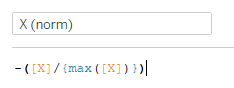
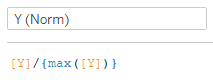
We already have the X,Y coordinates in the first viz, and as mentioned above, all we need to normalize it to be between -1 and 1 and fit the map environment, using LODs. The below calcs take the X and Y figures and compare them back to the max value of each yielding a ratio ranging from 0 to 1. A negative sign is placed before the X value as by default Tableau plotted these points counter clockwise.
Now we will create the MAKEPOINT function:

The next step is to drag it onto the details along with the song title field. We will also color the songs by the album colors:

Album Lines
Next, let’s create the album lines:

For the radial bars, we had an inner point and an outer point for each song which were connected by lines - this is what forms the radial bars (see Radial Bar blog). For the album lines, we will apply the same technique to create another MAKEPOINT using the X Norm and Y Norm we used for the songs, but we will only use the inner point.
The idea here is to place all the all the inner dots of the songs and then to connect them to each other using a the field (Point Det) which is simply a running index for each one of the songs by the order of appearance as shown below (I added it to the Label mark to emphasize how it works).

We will use a line chart type to and the Point Det field on the path card in order to connect the dots and create the album lines. Dragging the Album field onto the details will separate the lines per album.
So now we will need to create a new MAKEPOINT field (call it “makepoint album lines”), based on the same technique above but with a few changes. For the X (Norm) and Y (Norm) we used before, we will add the following changes:
- We will add an IF statement to keep only the inner points of the radial songs bar chart mentioned above so that it doesn’t extend out like the radial bar values do.
- We wish to create space between the song bars and the album lines. To do that, we will add a parameter to control the distance of the album lines from the radial song chart.

Now that we have a new make point, we will drag it onto the canvas to create a new layer for the album lines.

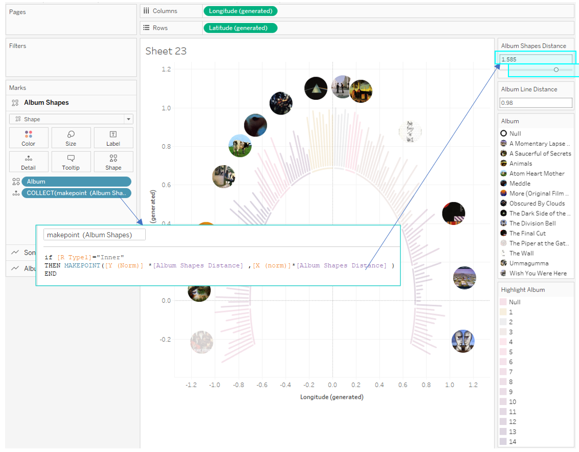
Album Shapes:
To go along with the album lines, I wanted to include some album shapes around the outside of the chart:

To do that, we will want to use the inner points again but now we want to place an album shape on top of each album song group.
We will create additional MAKEPOINT with additional parameters and now we will set it to be bigger than one as we want to create a bigger distance and push the inner dots out.
Note that now we will use only the Album field in the details (rather than the songs in the former 2 layers) as we want a single point for each album.
We will need a new MAKEPOINT field, quite similar to the former one but with another different parameter as we need more distance from songs lines layer:
Song Writers:
The last core part that we will focus on is the song writers layer. This was the most challenging layer and, in fact, ended up being 4 layers.

The data is structured with 4 columns for each song. Each of these columns indicates a writer, which could be any of the band members or “Other” (Note that there were no more than 4 different writers for any single song).
If a writer had exclusively written a specific song, all the columns would list his name.
In the case of 4 different writers, each column would list a different name.

So our goal here is to create a kind of radial stacked bar that will indicate the writer's contribution to each one of the songs.
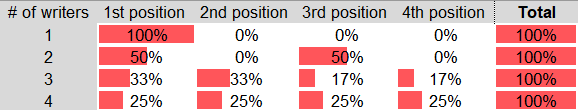
I already have the angle (from the radial song bar chart). Now I need to create a radius which length is determined according to the number of song contributors.
If I have a total length of 100%, I will need to allocate the length of each one of the positions according to the number of song writers:
Ultimately, this was a technical issue that had to be addressed and I don’t want to spend a lot of time focusing on it in this blog post (maybe in another one). Ultimately for each position, I had an angle and a length and needed to place one on top of another. I utilized parameters again.

Because I used 4 parameters for each one of the positions, songs with 3 writers was the most challenging. I could easily create logic for songs with 1 writer, 2 writers and 4 writers but 3 insisted not to align properly. After much struggle I found a way to resolve this by splitting the 3rd writer along the 3rd and 4th positions, and made it finally aligned. (I guess there is a more elegant way to achieve that). Again, I don’t want to dig too deeply into this.
I Implemented this logic in the data preparation stage yielding 4 sets of X, Y coordinates and lengths for each one of the 4 writers positions, thus 4 new sets of X (norm) and Y (Norm), we will need to create 4 additional MAKEPOINT fields (and as mentioned before) 4 parameters to set the distance:

We created 8 layers to cover the core elements of the central visual. In the final viz, I added more layers to add more fun elements (vinyl shapes, color highlights, faded shapes for selection highlighting, etc.). And all of this was completed on a single worksheet!
Now that the core elements completed let’s add some design.
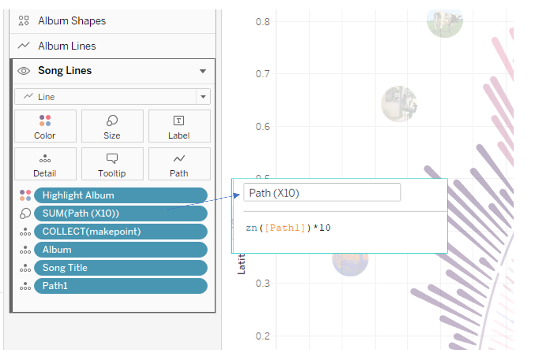
Songs Design Touches:
Let’s give the radial song bar chart a cone shape to resemble a light beam. To do that, we will use Path1 field (0 value for inner points, 1 value for outer points). But to make the effect more significant, we will multiply it by 10 in the Path (X10) field and drag it onto the size:
Now we will add faded circles on the end of the radial bar charts (the “light beams”) to resemble a spotlight by using the outer point of the radial bar charts. For that, we will create additional MAKEPOINT field (call it “makepoint outer”) and use an if statement to bring only the outer points:


We will use the same makepoint outer field to add the white note shape inside each one of the songs circles:

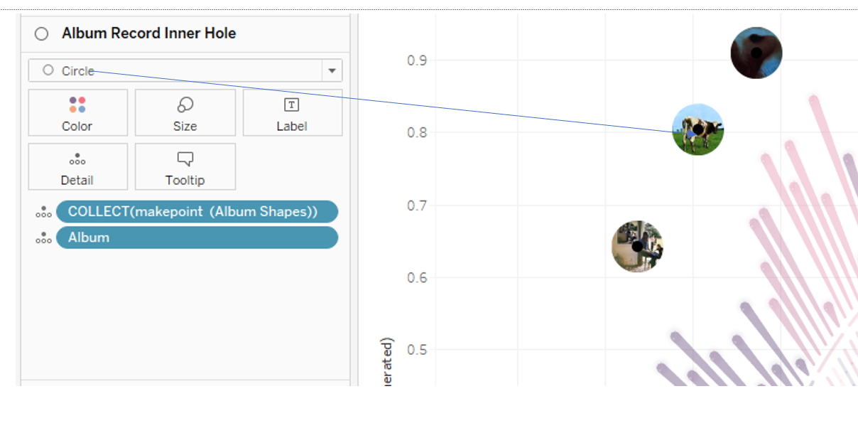
Albums Design Touches:
For the albums, let’s make them look a bit more like actual albums. First we will add a little hole inside each one of the album shapes by using a circle mark and the makepoint (Album Shapes) field we created for the album shapes.

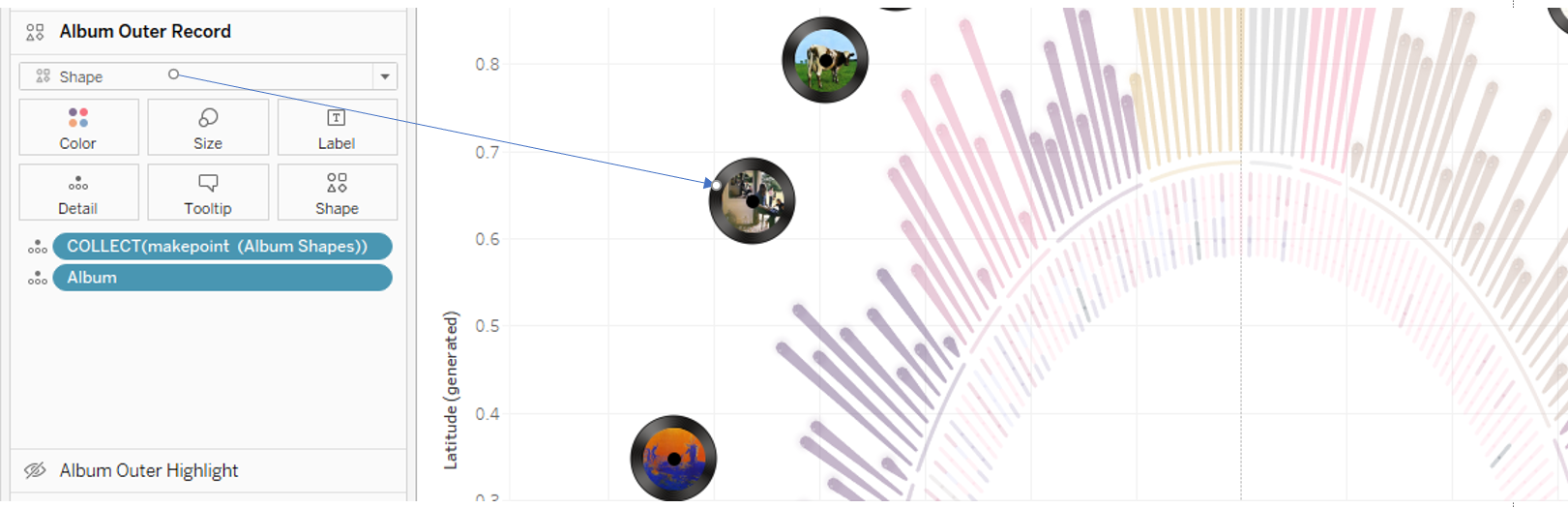
And we will use makepoint (Album Shapes) again to create a vinyl shape around the albums (using a custom vinyl shape):
And finally, we will add an outer glow to emphasize the album color by using a faded circle shape.

And there you have it! Our center view is ready using 17 layers!

Check out the original and the remastered version. I’m pretty excited about the improved design, but much more excited about the improved functionality and interactivity which was all made possible with map layers!

Well, that’s it. At first, the technique seems quite complicated, but after you walk through it a time or two, it becomes second-nature.
Thanks for reading and please feel free to contact me if you have any questions.
Nir
Kevin Flerlage, October 25, 2021
Twitter | LinkedIn | Tableau Public


Amazing work, Nir! Well deserved the spotlight!
ReplyDeleteYou are a Rockstar !
ReplyDeleteIndeed, first, I Love Pink Floyd, Love information perception and Tableau also needed to picture Pink Floyd for quite a while and this is the Viz I most appreciated making. This is actually so dop. every one of the collections and verses are together in one spot. This is truly perfect for Pink Floyd fans. I simply adored it. Much thanks.
ReplyDelete